
A Deep Dive Into The Concept of Regression
- Abhijit Roy
- Sep 26, 2020
- 10 min read


Regression is one of the most important concepts used in machine learning. In this blog, we are going to talk about different types of regressions and the underlying concepts. The variation in types of regressions are represented in the diagram:
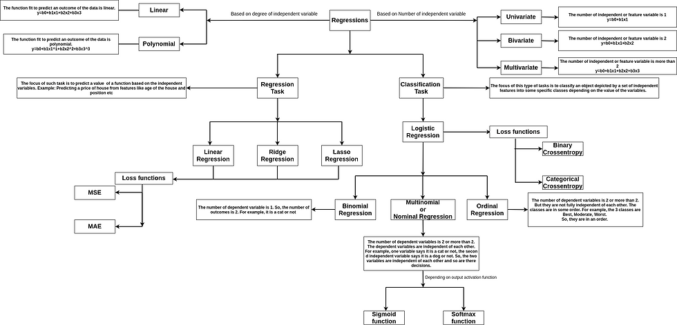
We are going to talk about all the points in detail.
Linear Regression
Regression tasks deal with predicting the value of a dependent variable from a set of independent variables i.e, the provided features. Say, we want to predict the price of a car. So, it becomes a dependent variable say Y, and the features like engine capacity, top speed, class, and company become the independent variables, which helps to frame the equation to obtain the price.
Now, if there is one feature say x. If the dependent variable y is linearly dependent on x, then it can be given by y=mx+c, where the m is the coefficient of the feature in the equation, c is the intercept or bias. Both M and C are the model parameters.

Say the red crosses are the points. X1 is the feature value, Y1 is the predicted value and Y_pred 1 is the actual target value. Here we can see the predicted and the actual value for X1 are the same. But, for X2 they are different. So, our job is to give the best fit line that exactly portrays the relationship between the dependent and the target variable. Now, first the model parameters M and C are initialized randomly, say M1 and C1 as shown in the figure given by line 1. It is evident that the line doesn't provide a very good fit. Then we move to line 2 given by parameters M2 and C2. This line provides a much better fit and acts as our regressor. It will not always give the exact fit but it gives the best possible fitting.
So, the question arises on how we reach from line 1 to line 2? The answer lies in the concept of cost function and gradient descent. To obtain the best fit line we train the model on a set of given values, which consists of the feature value and the corresponding target value (Y actual). So, we fit the feature value in the objective equation y=Mx+C. We obtain the Y_predicted value. Our target is to decrease the difference between the Y_predicted and Y_actual.
For the purpose, we use a loss function or cost function called Mean Square error of (MSE). It is given by the square of the difference between the actual and the predicted value of the dependent variable.
MSE=1/2m * (Y_actual — Y_pred)²
If we observe the function we will see its a parabola, i.e, the function is convex in nature. This convex function is the principle used in Gradient Descent to obtain the value of M2 and C2.
Gradient Descent
This method is the key to minimizing the loss function and achieving our target, which is to predict close to the original value.

In this diagram, we see our loss function graph. It has a specific global minimum which we need to find in order to find the minimum loss function value. So, we always try to use a loss function which is convex in shape in order to get a proper minimum. Now, we see the predicted results depend on the weights/coefficients from the equation Y=Mx +C or Y=Wx+C. The Weights in the X-axis and corresponding Loss value on the Y-axis of the graph. Initially, the model assigns random weights to the features. So, say it initializes the weight=a. So, we can see it generates a loss which is far from the minimum point L-min.
Now, we can see that if we move the weights more towards the positive x-axis we can optimize the loss function and achieve minimum value. But, how will the model know? We need to optimize weight to minimize error, so, obviously, we need to check how the error varies with the weights. To do this we need to find the derivative of the Error with respect to the weight. This derivative is called Gradient.
Gradient = dE/dw
Where E is the error and w is the weight.
Let’s see how this works. Say, if the loss increases with an increase in weight so Gradient will be positive, So we are basically at the point C, where we can see this statement is true. If loss decreases with an increase in weight so gradient will be negative. We can see point A, corresponds to such a situation. Now, from point A we need to move towards positive x-axis and the gradient is negative. From point C, we need to move towards the negative x-axis but the gradient is positive. So, always the negative of the Gradient shows the directions along which the weights should be moved in order to optimize the loss function. So, this way the gradient guides the model whether to increase or decrease weights in order to optimize the loss function.
The model found which way to move, now the model needs to find by how much it should move the weights. This is decided by a parameter called Learning Rate denoted by Alpha. the diagram we see, the weights are moved from point A to point B which are at a distance of dx.
dx = alpha * |dE/dw|
So, the distance to move is the product of learning rate parameter alpha and the magnitude of change in error with a change in weight at that point.
Now, we need to decide the Learning Rate very carefully. If it is very large the values of weights will be changed with a great amount and it would overstep the optimal value. If it is very low it takes tiny steps and takes a lot of steps to optimize. The updated weights are changed according to the following formula.
w=w — alpha * |dE/dw|
where w is the previous weight.
With each epoch, the model moves the weights according to the gradient to find the best weights.
Thus using the process we obtain the final values for the model parameters M2 and C2, which give us the actual best fit line.
Types of Regression
Univariate, Bivariate, and Multivariate
We have seen in the above instance we were representing the dependent variable as a function of a single independent variable, so we were using y=wx+c. This type of regression is called univariate as there is only one independent variable.
If there are two independent variables in the equation becomes:
Y=w1x1+w2x2+c
This is called bivariate regression.
Now if there are more than two independent variables i.e, the dependent variable depends on more than two features, the equation is modified accordingly.
Y=w1x1+w2x2+w3x3+…………..+wkxk+c

This is called multivariate regression.
2. Linear and Polynomial
Until now, we have seen linear regression problems, i.e, the degree for each independent variable is 1.
Now, if we have a non-linear curve like the one given below, we can’t draw

the best fit line, if we use linear regression. In such cases, we must opt for polynomial regression. Polynomial regressions raise the features or independent variables to powers and create a polynomial equation instead of a linear one. It is given as:
Y=w1x1¹ +w2x2² + w3x3³ +w4x4⁴ +………..+wkxk^k +c
Now, here the w1, w2, w3 ….. wk are the parameters of the model and the powers are the hyperparameters of the model. So, the degree of the polynomial is also a hyperparameter.
Say if y=ut+1/2gt² is a given equation, u and 1/2g are the model coefficients or parameters.
This is called polynomial regression.
Ridge Regression
Let’s consider a situation:

Now, here the red dots denote the points of the training set, and the blue dots denote the points of the test set. We can see if we train using the red points we will obtain the red line (1), as the regressor line, but it is very evident that the line (1) will have a very bad generalization and will not perform satisfactorily on the test data. This condition is said to have a high variance which leads to overfitting. This is where Ridge regression comes into play. It modifies the cost function and adds a regularization term. If we notice closely we will see that line (2) is a much better generalization and will perform better. The line (1) has very high weights and coefficient values for the equation:
Y=w1x1+w2x2+……………..+wkxk.
which causes the overfitting. The idea behind ridge regression is to penalize the sum of squares of the weights or coefficients to bring a regularization effect. Say, our equation is
Y_pred=w1x1+w2x2
The loss function becomes:
Loss= 1/2m.(Y_actual — Y_pred)² +lambda/2m. (w1² + w2²)
The second portion is the regularization portion, which focuses on penalizing the weights or coefficients and prevent them from achieving high values. As the function is our loss function, the gradient descent results in keeping a check on the weights also, as an increase in the weights in turn increases the loss function.
The lambda parameter is decided using cross-validation and is the measure of how much we focus on the regularizing our weights. The more the value of lambda, the more is the degree of regularization. So, lambda addresses a tradeoff.
This technique is also used in L2 regularization for Neural Networks.
Lasso Regression
The Lasso regression also addresses the same overfitting issue in Linear regression. The difference being in the way of modification of loss function. The Lasso Regression penalizes the absolute value of the sum of weights instead of the square of the weights.
If our equation is
Y_pred=w1x1+w2x2
The loss function becomes:
Loss= 1/2m.(Y_actual — Y_pred)² +lambda/2m. (|w1| + |w2|)
Now, here if the values of the weights are too small, they almost become equivalent to 0. If w2 is equivalent to 0, w2x2 becomes 0, this signifies that the feature x2 is not important for the prediction of Y.
Thus Lasso Regression is used for feature selection mechanism.
The same logic is used for L1 regularization for Neural Networks.
Classification Task
The type of task involves classifying an entity into some given classes based on a set of features. Logistic regressions is used for classification tasks.
Why not Linear Regressions?
Linear regressions normally is based on framing the best fit line. Let’s first see how can we use linear regression for classifications.

If we observe the above image ‘1’ denotes a class and ‘0’ denotes another. If we get the best fit line, and the dotted boundary(as shown), we can easily use it to classify. The blue points or 0 class when projected on the best fit line always give less than 0.5 which is the decision boundary value provided by the dotted line. Correspondingly, the 1 class or red points give values greater than 0.4.
Now, let’s look at the issues.
Let’s consider the below case:

Here, we can see the best fit line shifts due to the outliers which may create faults in classifications resulting in unsatisfactory results. Again, some points will give y value less than 0 and greater than 1. So, using linear regressions y can take values from -infinity to +infinity, but for classification problems, y must range from 0 to 1.
The above point are the reasons linear regressions can’t be used for classification tasks.
Logistic Regression
We know,
Y= w1x1+w2x2+w3x3……..wkxk
is used as the equation for linear regression.
Now, the values taken by the RHS -infinity to +infinity. So, we must transform the LHS also to range from -infinity to +infinity.
In order to achieve that we use log(Y/1-Y) as the LHS.
log(Y/1-Y)= w1x1+w2x2+w3x3……..wkxk
=>Y= 1/ 1+e^-(w1x1+w2x2+w3x3……..wkxk)
=> Y= 1/(1+e^-transpose(theta).x)
where, transpose(theta).x=(w1x1+w2x2+w3x3……..wkxk)
Now,
Y=1/(1+e^(- transpose(theta).x))
is also called Sigmoid Function, and it ranges from 0 to 1. Theta depicts the weight of coefficient vector or matrix and x is the feature matrix.

The above diagram shows the Sigmoid function. 0.5 is the boundary of the function, and it does not take value less than 0 and greater than 1.
Now, if sigmoid function is given by h(x) on the Y-axis, is a function of g(transpose(theta).x) on X-axis, then,
h(x)=g(transpose(theta).x)
We can derive the following,
h(x)>0.5
=>g(transpose(theta).x)>0.5
=> transpose(theta).x>0
Again,
h(x)<0.5
=>g(transpose(theta).x)<0.5
=> transpose(theta).x<0
So, if transpose(theta).x , i.e, w1x1+w2x2+w3x3……..wkxk >0 the entity is classified as 1 class else if w1x1+w2x2+w3x3……..wkxk <0, the entity is classified as a 0 class.
The decision boundary is given as shown:

The green line shows the decision boundary, and the equation represents the eqaution of the line. Now, from linear algebra, we know, if we pick a point (a,b,c,d) and fit it in the equation it will result in greater than 0 if it lies above the line, and less than 0, if it lies below the line. The analogy is very similar to what we saw above, class 1 if w1x1+w2x2+w3x3……..wkxk >0 and class 0 if w1x1+w2x2+w3x3……..wkxk <0.
This is how logistic regression works.
Loss function
In linear regression case, we used MSE or Mean Square Error. MSE is given by:
MSE=(Y_actual — h(x))²
h(x)=w1x1+w2x2+w3x3……..wkxk
In this case, MSE was a parabolic function and a pure convex one with a distinct minimum. But in this case,
h(x)= 1/ (1+e^-(w1x1+w2x2+w3x3……..wkxk))
Now, the modification of the cost functions distorts its convex properties and now there are multiple minima. In addition to it, if we use MSE the magnitude of error will be very less, (1–0)² =1 for maximum as the maximum value Y can take is 1 and minimum is 0, and so will be the penalty.
Owing to this region we use LogLoss or Binary cross-entropy for the purpose of logistic regressions.
Say, Y_pred=h(x), so, cost(h(x), Y_actual)=
— log(h(x)) for Y_actual=1 — log(1 — h(x)) for Y_actual=0
Combining the both the equation is framed as:
Loss= —Y_actual. log(h(x)) —(1 — Y_actual.log(1 — h(x)))
If Y_actual=1, the first part gives the error, else the second part.

The above diagram shows Log-Loss or Binary Cross-Entropy. If the label is 0 for actual and the predicted label moves towards 1, the loss function approaches infinity and vice versa. So, the loss is more and so is the penalty.
Types of Logistic Regressions
There are three types of Logistic Regressions,
Binomial Regression
Multinomial Regression
Ordinal Regression
The definitions are given in the diagram at the start. We will be talking about Binomial and Multinomial Logistic Regressions.
Binomial Regressions are those where the classification is done for two classes, say cats and dogs. It behaves in the same manner as discussed above.
Multinomial Logistic Regression or Multiclass Classification
In this case, there are multiple number of classes, an entity may be classified as. For example, there are four classes, Cat, Dog, and Lion. An image may be classified as any of the three classes. This is an example of multinomial classification. One thing to notice is, the three classes are independent of each other.
To solve these kinds we essentially convert multinomial Logistic Regressions to Binomial Regressions.
There are two approaches:
Simple Approach: The approach creates K Seperate logistic regression models for each of the K seperate classes. Each of the models has a sigmoid output node which denotes the output for that particular class. For our model, there will be 3 sigmoid nodes, 1st for cat, 2nd for dog and so on. Now, the 1st node gives the probability of the image being a cat P_c, the 2nd node gives the probability of the image being P_d, and similarly we obtain P_l for lion. Now, the scores are compared to obtain the final answers. If P_c has the maximum value among all 3, the image is predicted as a cat.
Simultaneous Approach: The approach creates K-1 Seperate Logistic regressions. Every probablity is proposed as a set of independent events, i.e, instead of a node deciding an image is cat or not(0/1), it decides the image is cat or lion (A/B).
Now, we have seen for logistic regressions:
log(Y/1-Y)= w1x1+w2x2+w3x3……..wkxk
If Y => 0.5 class A else class B. So, Y can be said P(A) and 1-Y is equivalent to P(C). This is called the Odds. So, for the first model:
log(P(A)/P(C))=w1_1x1_1+w2_1x2_1+w3_1x3_1……..wk_1xk_1+b_1
Say, R_1=w1_1x1_1+w2_1x2_1+w3_1x3_1……..wk_1xk_1+b_1 P(A)/P(C)=exp(R_1) — — — — 1
Again for the second model,
log(P(B)/P(C))=w1_2x1_2+w2_2x2_2+w3_2x3_2……..wk_2xk_2 + b_2
Say, R_2=w1_2x1_2+w2_2x2_2+w3_2x3_2……..wk_2xk_2 + b_2
P(B)/P(C)=exp(R_2) — — — — — -2
Now, from the above equations 1 and 2:
P(A)=P(C)*exp(R_1) P(B)=P(C)*exp(R_2)
Now, P(A)+P(B) +P(C) =1
So, P(C)*exp(R_1)+P(C)*exp(R_2)+P(C)=1
P(C)=1/(1+ exp(R_1) + exp(R_2))
Thus, we can inter relate among all of them.
Softmax Regressions
Softmax Regressions are given by:

The softmax layer is used as the final or output layer for multiclass classification. The function is an exponential approach. Sum of the probabilities of all the classes are equal to 1. The maximum probable class is given as output.
Conclusion
In this article, we have gone through all the concepts associated with regression. Hope this helps.


Comentários